UAV Geolocalization Using Satellite Imagery

• Motivation
• Geolocalization as an Image Matching Problem
• Aerial Cities Dataset
• Approach
  • Siamese vs Dual Network
  • Contrastive Loss Function
  • Training
• Results
• Examples of Correct Predictions
• Examples of Incorrect Predictions
• Conclusions
• Detailed Report

This post discusses the work I have done as a Masters Project at IIT Kanpur.

Motivation

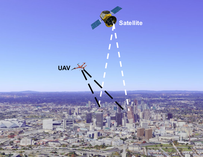
Recent advances in research in the field of unmanned aerial vehicles or UAVs have made them publicly accessible and relatively inexpensive. For most outdoor applications, UAVs generally rely on GPS to get a global pose estimate. However, for accurate geolocalization using GPS, the UAV must be able to receive a direct line of sight from four or more GPS satellites. This can be an issue in case of presence of high buildings, mountains or jammers which can obstruct the signals from satellites. So can we infer the global pose of the UAV without GPS? The answer is yes, we can use the camera sensors attached under the UAV to compare the scene with satellite images, and infer the location of the UAV.

Geolocalization as an Image Matching Problem

Consider a scenario where you have a database of satellite images annotated with their locations. By accurately matching an image from UAV camera with the database, one can get a good approximation of the latitude and longitude of the UAV.

In order to retrieve similar images from the satellite database, we must be able to accurately match satellite images with the UAV camera feed. So, in this work, we constrain ourselves to the problem of aerial image matching and train a deep learning model that can accurately match images from satellite and UAV camera.

Aerial Cities Dataset

In this work, we use the dataset introduced by this paper. This dataset is referred to as Aerial Cities hereafter.

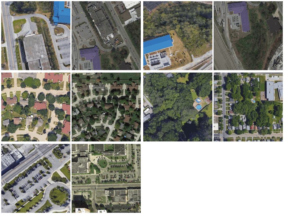
The UAV images are captured from Google Earth, and the satellite images are captured from Google Maps. The satellite images are always oriented towards the North ($0^\circ$ heading), and the images are taken from the camera facing the nadir. The UAV images have a random heading (between $0^\circ$ and $360^\circ$ ) and a random tilt from nadir (between $0^\circ$ and $45^\circ$ ). The UAV images have been taken from an altitude between $100m$ and $200m$ above the ground. The satellite images have been taken from an altitude of $300m$ above the ground.

Approach

Siamese vs Dual Network

In a siamese network, weights are shared between the two branches of the network. A dual network is simply a siamese network with unshared weights.

Dual network has twice the number of parameters as compared to a siamese network with the same backbone. It has a separate feature extractor for each image distribution (eg, we have images from two distributions: UAV and satellite), which allows the network to learn richer features for each of the distribution.

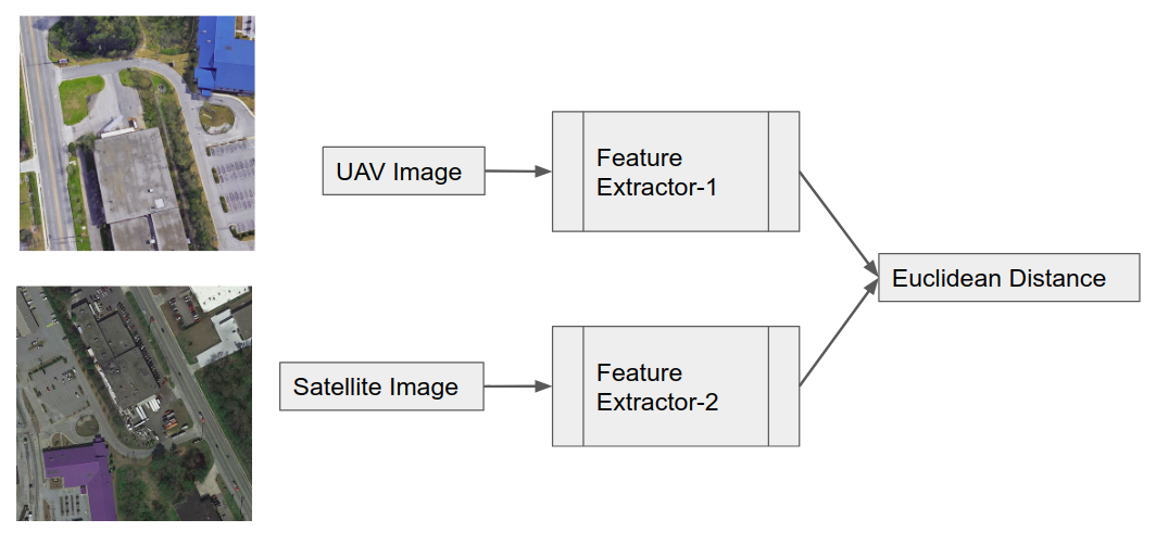
In this work, we found out that for this particular problem, a dual network works better than a siamese network. For training the network, we used contrastive loss function.

Contrastive Loss Function

$L = l \times d^2 + (1-l) \times (\max (0, m-d))^2$

where $L$ is the loss function, $l$ is the label ($l=1$ for matching pairs, and $l=0$ for non-matching pairs), $m$ is the margin and $d$ is the distance between image features, which is the output of the network.

For matching images, $l=1 \implies L = d^2$.
For non-matching images, $l=0 \implies L = 0$ if distance is greater than the margin. However, if the distance is less than the margin, the loss is $L=(m-d)^2$.

For our experiments, we set $m=100$.

Training

We follow the 5 step approach given below to train our networks.

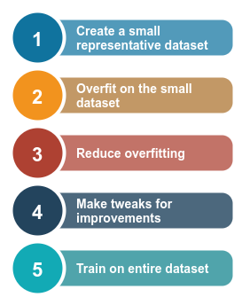
1. Creating a small representative dataset allows us to test some of our approaches quickly and identify the methods which will work well. For example, during our experiments we found out that a network pretrained with imagenet weights train much more quickly as opposed to the uninitialized one (read Kaiming Normal).
2. Overfitting serves as a sanity check and demonstrates that our network is actually learning from out training set. It shows that the chosen strategy is good enough for our task.
3. Overfitting can bee easily reduced by using more data, using data augmentation techniques and adding regularization.
4. As we are using transfer learning, some tweaks like discriminative layer training and gradual unfreezing can make sure that the initial layers which can identify fundamental features like blobs, corners, colour gradients and simple patterns are not disturbed while training.
5. After finalizing the strategy we are ready to train on the entire dataset.

In order to read more about the experiments, download the report project at the end of this post.

Results

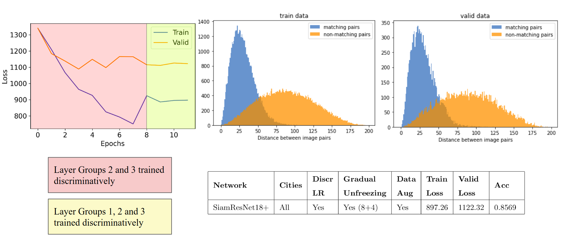
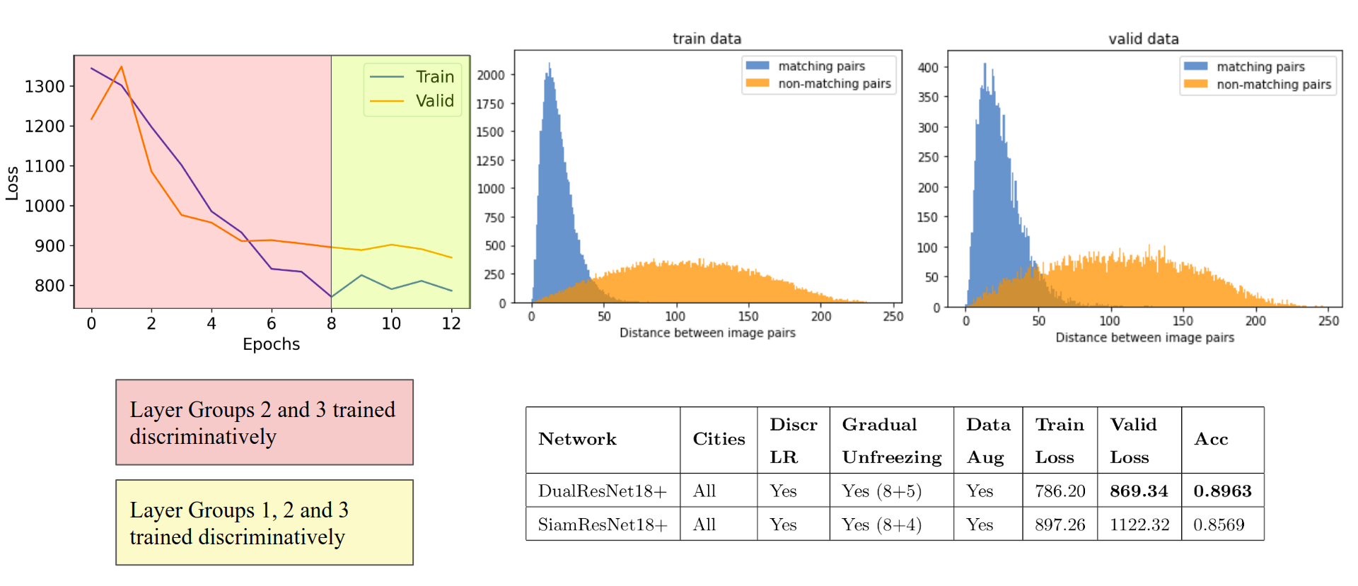
Our experiments show that the dual network performs slightly better than siamese network. The reason behind it is that the dual network architecture can learn from two specific distributions. The first diagram below corresponds to siamese network, while the second one corresponds to dual network.

Examples of Correct Predictions

The figure below shows a true positive: the matching pair which was actually predicted as matching. While testing, if the output distance comes out to be less than 50, we call the pair matching. This is because during training, we set the margin $m=100$.

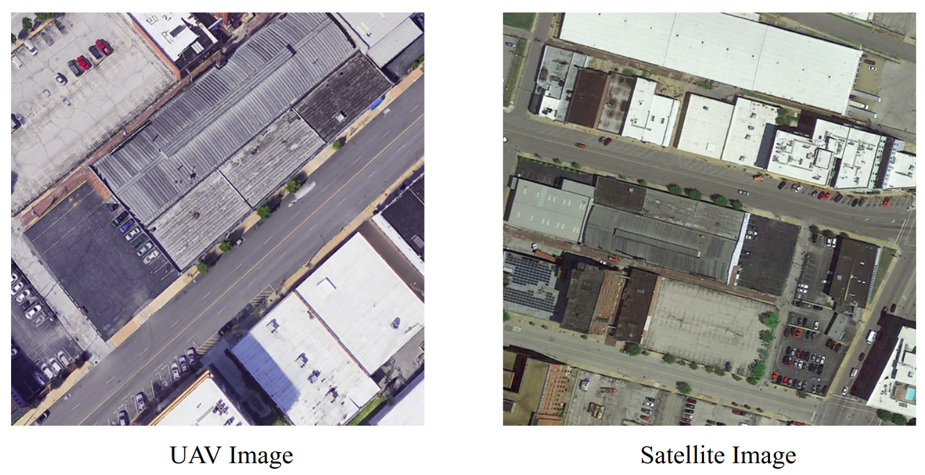
Looking at the images above, one can clearly notice that predicting whether two images are of the same geographic scene is not a trivial task.

Examples of Incorrect Predictions

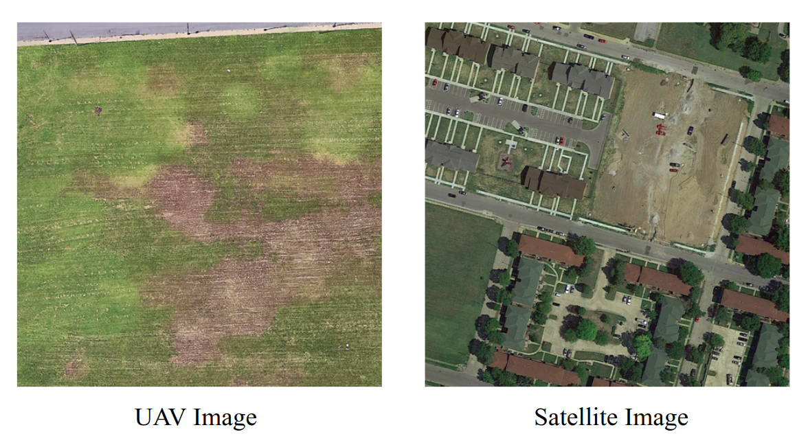
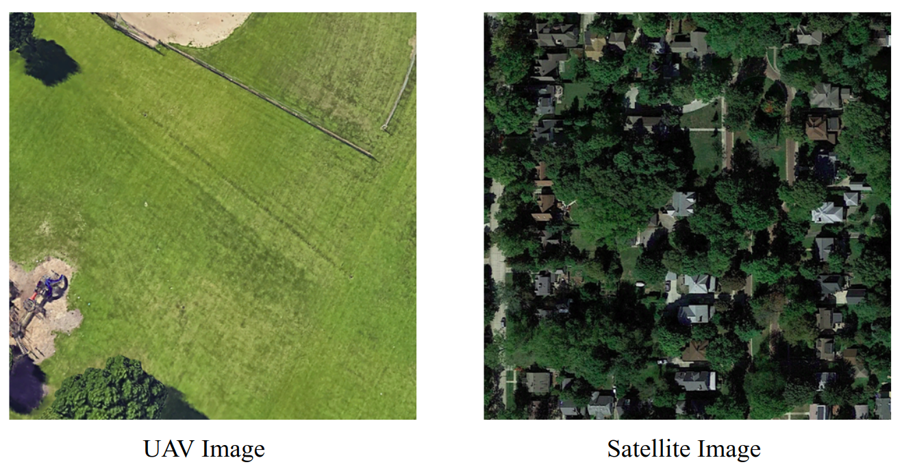
The model predicts the first example as non-matching. However, it is actually a matching pair. (False Negative)

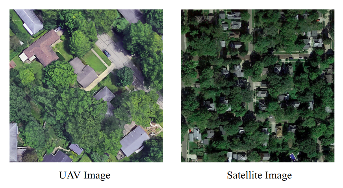
This is a very hard example. The model predicts this second example as matching. However, it is actually a non-matching pair. (False Positive)

Conclusions

The examples on which the model fails are very confusing even to human eye. The model gets confused when:

• the major portion of a UAV image is covered with a single structure
• there is a lot of greenery or repeated city structures in the images

Dual networks are superior to siamese networks when the data comes from 2 specific distributions, our model has the ability to correctly predict same scene or not 9 times out of 10.

Detailed Report

You can read the entire report by downloading it here. You may also view the code on the project repository.